Welcome to the Analysis Plus Knowledge Base. Here you’ll find a wide variety of useful and valuable materials and information to help you understand how and why you can benefit from our patented audio products.
Analysis Plus provides leading-edge research and technology in the field of electronic systems and components. Many of our customers are major names in high-end audio and home theater equipment. These manufacturers rely on us for our skills, reputation, and expertise during all phases of product development.
Our recent innovations in audio cable design were prompted by the realization that we could substantially improve the state-of-the art in cable design and performance. Along with our background in electrical engineering, we are also audiophiles and wanted to create the best cables available anywhere–period!
What Makes a Good Cable?
While testing audio cables for several well-known manufacturers, we learned that their criteria for what supposedly made one cable perform better or worse than another was remarkably inconsistent. One manufacturer’s claims countered and negated the claims made by a different manufacturer. Yet each one purported to be the best! As we studied the available literature, we quickly realized that the source of the problem was a lack of hard evidence supporting all the hype. None of the manufacturers offered documented, measurable evidence that it was producing a superior cable. Instead, we found claims of allegedly superior components or materials used in cable construction.
For example, a few leading manufacturers claimed that the most important factor for a cable was low capacitance, using the justification that cable capacitance shunts upper frequencies to ground. In order to lower the capacitance, these companies increased conductor spacing to simultaneously achieve a goal of increased inductance. This approach had drastic side effects, however. Merely decreasing capacitance without taking other realities of signal transmission into consideration increased the noise pickup and introduced a blocking filter. Both of these effects would obviously degrade sonic performance rather than improving it.
Another cable manufacturer advertised that its cable “employs two polymer shafts to dampen conductor resistance”, but offered no evidence to prove it. Still another audiophile company claimed that because its cable was flat, “with no twist, it has no inductance”. In general, inductance can indeed be reduced by making conductors larger or bringing them closer together. However, physics shows that, in reality, no cable can be built without some level of inductance, so this claim is without scientific merit.
To convey musical information effectively, a cable must provide a structured, low impedance path for the desired signal. This became our goal at Analysis Plus, Inc. We began by applying our expertise in electromagnetic computer simulation and design to rigorously test and study a broad range of audiophile cables currently on the market. Based on what we learned, we then set about designing our own approach to audiophile cables, relying on solid, measurable data rather than subjective claims.
Cylindrical Cable Conductors and Skin Effect
Most of the popular loudspeaker and musical instrument cables on the market employ cylindrical (a.k.a. round-diameter) cables as conductors. Unfortunately, cylindrical cable designs have a number of serious drawbacks, including current bunching, skin effect phenomenon, and frequency effects that lower the performance of the cable.
It’s a common misconception to think about electrical transmission in cables in terms of direct current (DC) alone. Even experienced electrical engineers frequently ignore the ramifications of frequency on cable performance. In the case of DC, current is indeed uniformly distributed across the entire cross-section of the wire conductor, and the resistance is a simple function of the cross-sectional area (see figure 1a). Adding the frequency of an electrical signal to the equation complicates the situation, however. As frequency increases, the resistance of a conductor also increases due to skin effect.
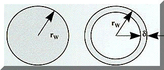
Figure 1a (left) and 1b (right) is of a round cable showing the effect of skin depth where Rw is the radius of the wire and is the skin depth. The shaded region represents the current density.
Skin effect describes a condition in which, due to the magnetic fields produced by current following through a conductor, the current tends to concentrate near the conductor surface (see figure 1b). As the frequency increases, more of the current is concentrated closer to the surface. This effectively decreases the cross-section through which the current flows, and therefore increases the effective resistance.
The current can be assumed to concentrate in an annulus at the wire surface at a thickness equal to the skin depth. For copper wire the skin depth vs. frequency is as follows:
60 Hz = 8.5 mm, 1kHz =2.09 mm, 10 kHz =0.66 mm, 100 kHz =0.21 mm.
Note that the skin depth becomes very small as the frequency increases. Consequently, the center area of the wire is to a large extent bypassed by the signal as the frequency increases (see Figure 2b). In other words, most of the conductor material effectively goes to waste since little of it is used to transmit the signal. The result is a loss of cable performance that can be measured as well as heard.
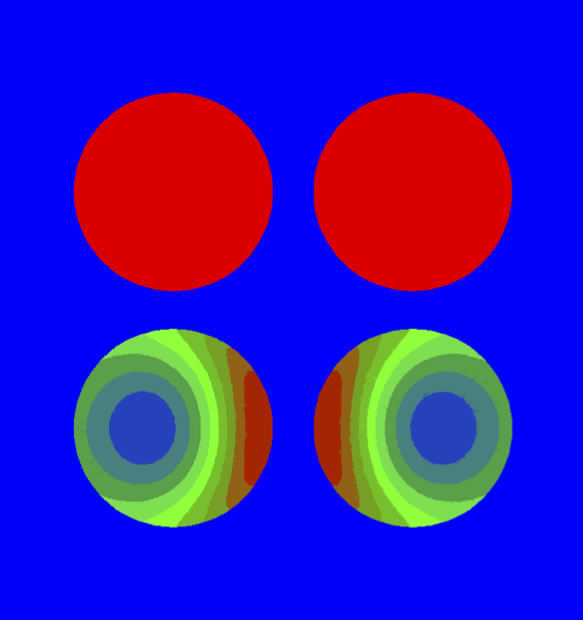
Figure 2a (top) shows uniform current distribution at DC. Figure 2b (bottom) shows the effect of current bunching and skin effects at 20kHz.
Current Bunching
Current bunching (also called proximity effect) occurs in the majority of cables on the market that follow the conventional cylindrical two-conductor design (i.e., two cylindrical conductors placed side-by-side and separated by a dielectric).
When a pair of these cylindrical conductors supplies current to a load, the return current (flowing away from the load) tends to flow as closely as possible to the supply current (flowing toward the load). As the frequency increases, the return current decreases its distance from the supply current in an attempt to minimize the loop area. Current flow will therefore not be uniform at high frequencies, but will tend to bunch-in. This can be seen in Figure 2b, which illustrates typical current density distribution in a cross-section view of a pair of cylindrical 12-gauge wires at 20 kHz. The density shadings are shown in color, with red being the highest current density and purple the lowest current density.
The current bunching phenomenon causes the resistance of the wires to increase as frequency increases, since less and less of the wire is being used to transmit current. The resistance of the wire is related to its cross-sectional area, and as the frequency increases, the effective cross-sectional area of the wires decreases. In order to convey the widest frequency audio signal to a loudspeaker, you want to use as much of the conductor cross-section as possible, so excessive current bunching is extremely inefficient.
Disadvantages of Rectangular Conductors
As a means of bypassing the skin effect and current bunching problems associated with cylindrical conductor designs, some cable manufacturers have developed rectangular conductors as an alternative. These designs typically use a one-piece, solid core conductor.
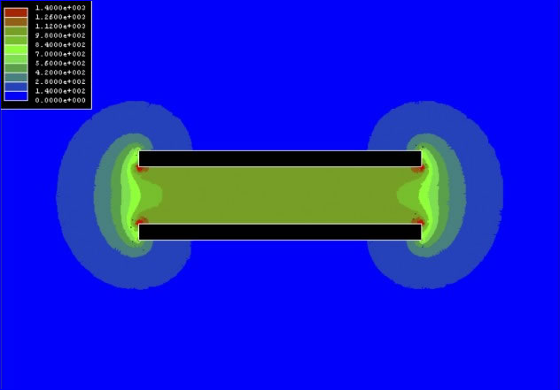
Figure B
Computer simulation showing the magnitude (volts/meter) of the electric field between two solid rectangular conductors. The conductors have a cross section area equivalent to a 10 gauge conductor. The spacing between the two conductors is 2mm with a voltage of +1 volt applied to the top conductor and -1 volt applied to the bottom conductor.
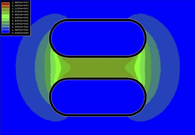
Figure C
Computer simulation showing the magnitude (volts/meter) of the electric field between two hollow oval conductors. The conductors have a cross section area equivalent to a 10 gage conductor. The spacing between the two conductors is 2mm with a voltage of +1 volt applied to the top conductor and -1 volt applied to the bottom conductor.
A solid rectangular conductor of this type is undesirable because the sharp corners produce high electric field values that over time can break down the dielectric, causing a failure of the cable (see Figure b). In general, cables with solid conductors are prone to shape distortions and kinking due to their poor flexibility. This becomes an especially important issue with rectangular cable designs. The sharp corners from rectangular conductors tend to chafe the cable dielectric if the cable is repeatedly flexed or put under stress, and this chafing can lead to a short that could conceivably damage your loudspeakers.
The Hollow Oval Cable Solution
After many computer simulations and other exhaustive tests, the engineers at Analysis Plus reached an innovative solution that flew in the face of conventional wisdom on audio cable geometry. Our engineers determined that a hollow oval cable constituted the best possible conductor design. Here’s why.
The primary advantage of an oval conductor design rather than cylindrical conductor geometry is that the oval shape allows more of the return current to be closer to the outgoing current, thus reducing the negative effects associated with excessive current bunching.
Figure 1 illustrates that at DC the current is uniformly distributed across the cross-section of the wire, but as the frequency gets higher, the current is distributed near the surface. Since the center part of the conductor is not used at high frequencies, we can simply eliminate it. By using a hollow conductor, we help minimize the change in resistance with frequency and the cable becomes more efficient.
Advantages of a Braided Conductor
Along with the innovative hollow oval conductor design in our Oval cable product line, we also determined that a braided conductor was superior to solid core conductors for two significant reasons.
The most obvious advantage of a braided conductor is that it yields a more mechanically reliable cable than solid conductor designs. A woven or braided cable is more flexible and resistant to stress fractures resulting from continual flexing than a solid cable. A solid cable is also more susceptible to kinks and other deformations when handled. Our cable can be handled easily, and it returns to its original shape when flexed. The flexibility of our cable also prevents the geometry of the conductors from changing with use. If the geometry changes, the cable characteristics will change, and kinks will add impedance mismatches–inducing distortion in the signal.
Braided cable has yet another advantage over solid core conductors. Analysis Plus, Inc., uses a woven pattern in its Oval cables where every wire is statistically as close to the return current as every other wire. The current density is now more evenly distributed between the strands. As a result, the resistance of our Oval cables is extremely constant over a variety of frequencies–much more so than solid-core cylindrical cables, as can be seen in Figure 3.
Characteristic Impedance Complexity
Another parameter that is critical in cable design is characteristic impedance. But because of its complexity, this important factor is often misunderstood.
The characteristic impedance of a cable is given by Z = [(R + jwL)/(G + jwC)]1/2 where R is the series resistance, L is the series inductance, G is the shunt conductance, C is the shunt capacitance, and w is the angular frequency (w = 2pief).
Note that this is not a simple number for a cable, but one which changes with frequency. It is also important to note that R, L, G, and C also change with frequency, making the impedance of a cable even more frequency dependent.
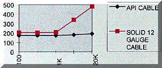
Figure 3
Frequency Hz | R vs.f Measured with HP 4263A LCR meter
Z is a complex number, and it is common practice in the cable industry to simplify the situation by assuming a loss less transmission line and, in turn, assuming that R and G are zero. While this may be a valid approximation at high frequencies, it is not valid at low audio frequencies if you plan to construct an accurate model of a cable.
For example, stating that a speaker cable has a constant, characteristic impedance of 10 ohms across the entire frequency range of 20 to 20,000 Hz is a drastic oversimplification that, in the end, is simply untrue. The same type of statement is also inaccurate when applied to loudspeakers, as the table below shows. A speaker only has a constant impedance of 8 ohms at a single fixed frequency. To state otherwise is to ignore the complexity of impedance changes as signal frequency changes.
Measured Speaker Impedance (Ohms)
| Speaker | 100 Hz | 1 kHz | 10 kHz | 20 kHz |
|---|---|---|---|---|
| EPI 100 | 4.5 -13.8 deg | 12.8 +9.8 deg | 6.26+13.8deg | 8.01+29.2deg |
| Bose 901 | 16.5+49.1deg | 8.72+15.9deg | 26.4+47.5deg | 26.4+47.5deg |
| JBL TI 250 | 6.17-14.4deg | 10.4-2.1deg | 5.22-13.4deg | 6.10+6.41deg |
Minimizing Impedance Mismatch
Our Oval cables minimize frequency changes and boast a low impedance to reduce reflections at the high end of the audio frequency range.
Conventional cylindrical cable, due to its geometric limitations, typically has an impedance of about 100 ohms at the high end of the audio frequency band, thereby causing an impedance mismatch at high frequencies. In an attempt to eliminate impedance mismatch, some audiophile cable companies introduce passive components into their cables. However, these components can do more harm than good by introducing another possible source of pollution (or distortion) to the signal.
As shown in Figure 3, Analysis Plus Oval cables minimize the change in resistance with frequency. Our exclusive braided conductor, hollow oval design also minimizes the frequency dependence of the inductance L as shown in Figure 4. By minimizing current bunching and skin depth problems, we minimize unwanted distortion, maximizing transparency and realism.
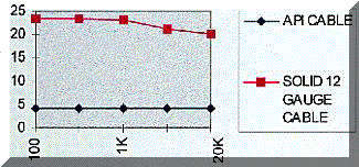
Figure 4
Frequency Hz Ls vs. f | Measured with HP 4263A LCR meter
Frequency Blurring
To minimize frequency blurring, it is important that the speaker cable parameters do not change with frequency. Ideally, the resistance and inductance would remain constant as the frequency of the signal changes. Figure 3 and 4 show that Analysis Plus, Inc., Oval cable minimizes the change of R and L with shifts in frequency, thus minimizing frequency blurring.
Wave Good bye to EMI
Electromagnetic Interference (EMI) is commonly encountered when multiple electronic devices are operated in close proximity to one another. Almost everyone has heard or seen the interfering effect of a vacuum cleaner, lawnmower engine, hair dryer, or blender on a radio or television. These are examples of EMI, which can also significantly degrade the performance of a hi-fi system. How does EMI get into your system? AC wiring is one route. But even when this entry point is eliminated by using power conditioning components, EMI still gets into the signal path. Speaker cables are frequently the culprit.
As discussed on page 29 of Henry W. Ott’s Noise Reduction Techniques in Electronic Systems, loudspeaker cables generally comprise the longest parts of a system and therefore act as antennae that pick up and/or radiate noise.
While all real-world cables fall short of ideal behavior in eliminating the problems of EMI, our Oval cables perform closer to the ideal than any other cable currently on the market. To reduce EMI, it is important to have a low inductance. Our Oval cables exhibit low inductance which helps reduce noise and therefore improves the final sound.
Figures 5 and 6 show the superiority of Analysis Plus cable to other cable designs. The two plots in the graph represent measured data taken using a digital oscilloscope and a signal generator to produce a test signal. The purple waveform shows the source signal at the amplifier. The green waveform shows the signal after transmission to the speaker through a cable. For best performance, a cable should not distort the signal–the source signal and the signal at the speaker should show similar if not nearly identical waveforms.
1 1.00V 2 1.00V 0.00 10.0 2 RUN
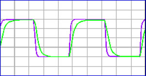
Figure 5
Purple / Green showing signal at speaker using OMC cable.
Figure 5 shows that the leading large-diameter audiophile cable greatly distorted the signal that the speaker receives. (Note the difference between the purple and green waveforms). Figure 6, in marked contrast, shows that a signal passed through the Analysis Plus, Inc., Oval cable to the speaker is essentially identical to the signal at the amplifier.
1 1.00V 2 1.00V 0.00 10.0 2 RUN
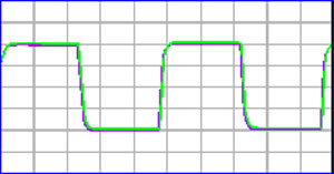
Figure 6
Purple showing signal at amplifier. Green showing signal at speaker using API speaker cable.
Imagine how much music you’ve been missing simply due to inferior cable!
The Best Test Instrument–Your Ears
Finally, we turn our attention to human hearing. After all, our end goal at Analysis Plus, Inc., is to bring our customers the best sound possible, and your ears are the ultimate judges of our success.
The faintest sound wave a normal human ear can hear is 10(-12) Wm(-2). At the other extreme of the spectrum, the threshold of pain is 1 Wm(-2). This is a very impressive auditory range. The ear, together with the brain, constantly performs amazing feats of sound processing that our fastest and most powerful computers cannot even approach.
As long ago as 1935 Wilska 2 succeeded in measuring the magnitude of movement of the eardrum at the threshold of audio sensitivity across various frequencies. At 3,000 Hz, it takes a minimal amount of eardrum displacement (somewhat less than 10-9 cm or about 0.01 times the diameter of an atom of hydrogen) to produce a minimal perceptible sound. This is an amazingly small number! The extremely small amount of acoustic pressure necessary to produce the threshold sensation of sound brings up an interesting question. Does the limiting factor in hearing minimal level sounds lie in the anatomy and physiology of hearing or in the physical properties of air as a transmitting medium?
We know that air molecules are in constant random motion, a motion related to temperature. This phenomenon is known as Brownian movement and produces a spectrum of thermal-acoustic noise.
In 1933, Sivian and White experimentally evaluated the pressure magnitudes of these thermal sounds between 1kHz and 6 kHz. They observed that throughout the measured spectrum the root-mean-square thermal noise pressure was about 86 decibels below one dyne per square centimeter. The minimum root-mean-square pressure that can produce audible sensation between 1 kHz and 6 kHz in a human being with average hearing is about 76 decibels below one dyne per square centimeter, but in some people with exceptionally acute hearing may approach 85 decibels.
These figures indicate that the acuity of persons possessing a high sensitivity of hearing closely approaches the thermal noise level, and a particularly good auditory system actually does approach this level. Furthermore, it is not likely that animals possess greater acuity of hearing in this spectrum, as their hearing would also be limited by thermal noise.
What this means is that the human audio system is extremely sensitive, and that small things like cable design are important to maximize the listening pleasure. At Analysis Plus, Inc., we’re committed to doing our part by bringing you the best-sounding audiophile cables on the market.
References
1 Henry W. Ott, Noise Reduction Techniques in Electronics System (New York, NY John Wiley and Sons, 1988, p. 150)
2 Wilska, A.: Eine methode zur Bestimmung der Horschwellenamplituden des Trommelfells bei verschiedenen Frequenzen, Skandinav. Arch. Physiol., 72:161, 1935.
3 Sivian, L.J., and White, S.D.: On minimum audible sound fields, J. Acous. Soc. Am., 4:288, 1933
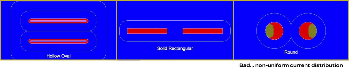
The following slide show is the first finite element computer simulation ever done looking inside 3 different copper conductors geometries. You are looking at the current inside a cross section of 3 different wires at different frequencies. Before this we use to guess what the current looked inside a conductor and talk about skin effect but ignore the proximity effect because we could not model it. Read our white paper for more detail.
Why do Hollow Oval cables sound better?
As the frequency is raised to 4 kHz, non-uniform current distribution appears in the round conductor cable. This change alters the resistance and inductance properties of the cable, an unwanted effect.
Why do Hollow Oval cables sound better?
The plots at 10 kHz show increased areas of reduced current density for both the rectangular and round geometries. The effect is much more pronounced for the round conductor, which leads to greater changes in its electrical parameters.
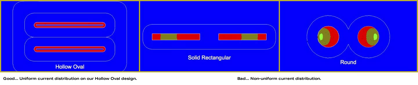
With our Hollow Oval design, note the uniform current distribution, even at 20 kHz. This is why the electrical properties of the Analysis Plus cables don’t change, and why more of the music is delivered to your speakers and to your ears.
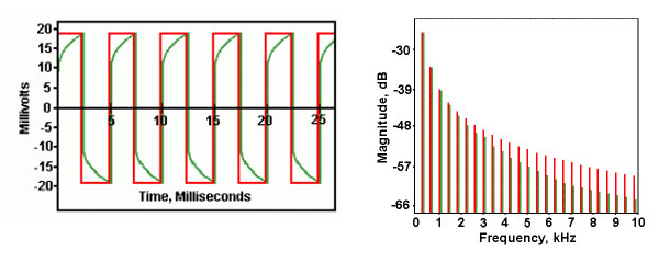
Why is it important that a cable’s electrical properties don’t change over the audio frequency band? Let’s look at the simple case of a square wave. The plots on the left will be time signals, like one would view on an oscilloscope. A time-domain waveform can also be represented in the frequency domain. This field of study is known as Fourier analysis. The frequency plots will be shown on the right.
Here are the representations of a 200 Hz square wave:
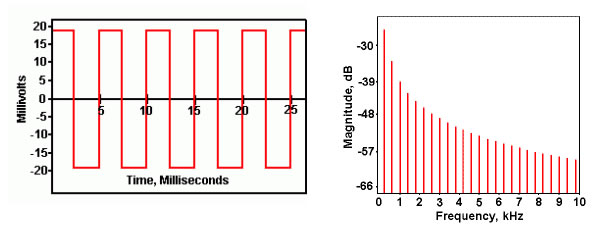
If we pass this square wave through a perfect cable, we would get back all the frequency components exactly, which means we’d see exactly the same square wave, just delayed a bit in time, depending on the cable’s length. In the frequency domain, we’d see the same magnitudes as before. The only change would be in phase, which we’re not plotting.
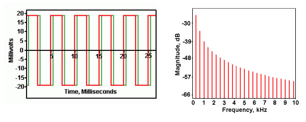
If we passed the signal through a cable which attenuated the signal somewhat, but uniformly across the audio band, we would still see a square wave, but one which was reduced in amplitude. The essential character of the signal remains the same, it’s just not quite as loud. We could compensate for the difference from the perfect cable by simply increasing the amplification.
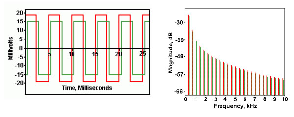
What happens when the attenuation is not uniform, but rather, varies with increasing frequency? We see that the shape of the time domain waveform is altered. For a simple square wave, we see that the shape is no longer square, but has corners that are rounded over. The essential nature of the time domain waveform is changed, and we can no longer recover the original signal by simply increasing the amplification.
How does this apply to the music we hear? A square wave has a very simple waveshape when compared to the complex signature of a musical passage. A piece of music is made up of a fundamental frequency plus a whole host of other frequencies, known as harmonics. It’s this harmonic content that allows us to distinguish one instrument from another, and to tell one person’s voice from another person’s.
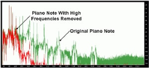
Below are two sound clips, both of the same piano note. One is the original note, the other has had much of the high frequency content removed. Comparisons of the two signals are shown in the plots below.
Hear original piano notes
Now hear piano notes with high frequencies removed
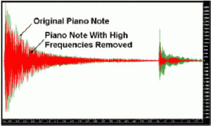
If we alter the frequency spectrum in a non-uniform way, we alter the harmonic content and hence the essential time waveform. We’ve changed the character of the music we hear.
Although exaggerated for web purposes, these sound clips show what happens when sound data is lost. This loss of high frequency information is one of the main reasons cables sound different. Analysis Plus cables were specifically designed to minimize the loss of high frequency information, and that’s why they sound better.
That’s why Analysis Plus Hollow Oval cables sound better! Through the use of computer modeling, we’ve designed a cable through which the current distribution changes very little over the audio band. This means that the electrical properties of the cable, its resistance and inductance, don’t change with frequency. The result is a cable that transfers the electrical energy from your amplifier to your speaker, without altering the time domain waveform of your music. You hear everything the musicians intended.
NASA contacted a number of high end audio cable manufacturers, searching for an ultra high quality flexible cable to allow one of their lasers to be mobile. Our Big Silver Oval and Solo Crystal Oval speaker cable were the only cables which met NASA’s specs for things like rise time and low impedance, under extremely demanding loads. We are very proud to provide NASA with our cables. This is the letter we received after their initial testing.
Hey Mark,
Searching the speaker wire industry for an appropriate transmission line has been difficult with the rarely posted figures.
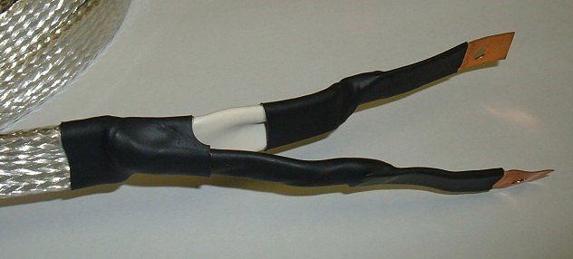
I appreciate the fast response and shipping. They arrived on Friday, but only yesterday did I get to test the wire types. I unbraided the very ends and attached a stub of flat copper so that I could bolt them on our posts.
Our operating condition was 250us to 1ms 120A current pulses at 80V into our laser diodes. That puts our load impedance below an ohm. I’ve attached a photo of the silver oval prepared. The wires performed very well and are a viable substitute for the stiff flat we currently use. The output of Big Silver Oval looked the best and is most similar to our flat wire. Silver Oval 2 showed a little bit of oscillation at the beginning of each pulse but was well within a stable range. These are the only two speaker cables we have tested that meet our requirements. I like that its nearly as small as our flat also (which is 10mm x 2mm).
No the application is not confidential. The laser’s a high energy, narrow line-width 2um pulse. It can be used for wind profiling, CO2 measurements, and other things. If you need something official though, I’d probably need to talk with others.
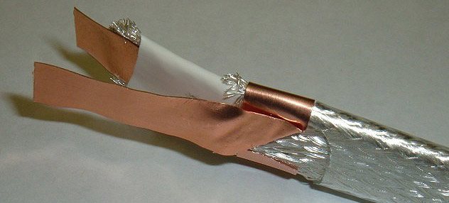
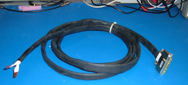
I can provide some (attached) but you’ll see in our final assembly that you can’t see the cable itself. We had to wrap it in a neoprene insulator for protection and requirements. We have three sets of these for our system (3 laser pump sources). The cable does work very well for our application. The clamp image is how we translate the oval cable to a high current connector. Our length is about 10 feet.
Will order 100 ft of Big Silver Oval to ship to NASA, LaRC, Building 1202, Room 223, Mail Stop 488, 5 North Dryden Street, Hampton, Virgina 23681.
Hope that helps,
Paul
Paul J. Petzar
National Institute of Aerospace